
Boosting Selection Of Most Similar Entities In Large Scale Datasets
TL;DR
Comparing very large feature vectors and picking the best matches, in practice often results in performing a sparse matrix multiplication followed by selecting the top-n multiplication results. In this blog, we implement a customized Cython function for this purpose. When comparing our Cythonic approach to doing the same with SciPy and NumPy functions, our approach improves the speed by about 40% and reduces memory consumption. The GitHub code of our approach is available here.
Introduction
ING Wholesale Banking has huge amounts of data about many companies, but because the data comes from different source systems, inside and outside the bank, there is no single identifier that can be used to easily connect the data sets. Therefore, we have to connect the data sets based on the names of the companies in the different sets, which are often written in different ways.
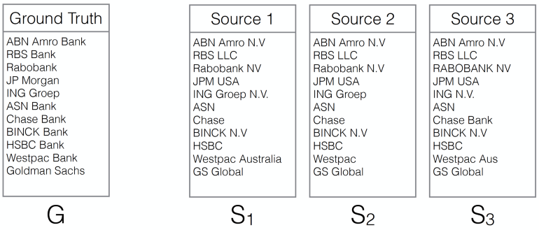
Figure 1 shows this name matching problem conceptually. Depending on the use case, the two data sets of names to be matched can be up to 10 million and 100 million names respectively. There are many ways to look at the problem, such as an approximate string matching problem, nearest neighbor searching problem, pattern matching problem, etc. We opt for a method that does tokenization and cosine similarity searching, because:
- It is fast: the main computation is matrix multiplication, and SciPy and NumPy facilitate fast matrix computation. The computation of tokenization and vectorization can be easily parallelized.
- It is accurate: a tokenizer can make the matching order unrelated and fuzzy, which means an accurate method.
Our colleagues Wendell Kuling and Chris Broeren gave a presentation on this in a PyData meetup.
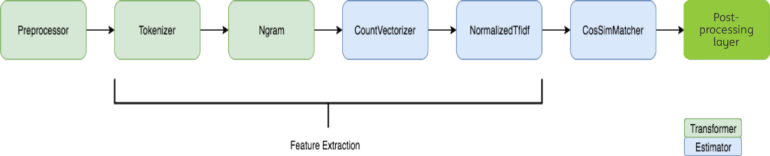
As shown in Figure 2, we implement the whole pipeline in Spark ML pipeline, which is elegant and fast (another post will discuss it). A preprocessing is done in order to reduce the noise in the names. TFIDF features (Wiki page) are extracted for the names to represent them in vector format. Cosine similarity is used as the similarity metric between these vectors to find top n candidates. Among the selected candidates, the best match is found by a supervised method.
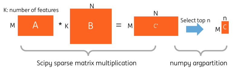
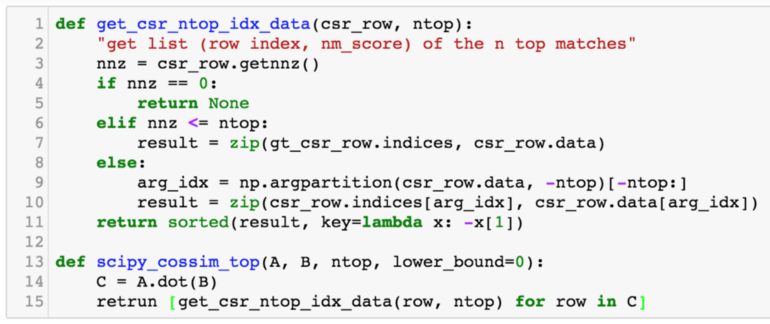
It is noted that a very sparse matrix is generated after the vectorization. The feature space is 16 million (the vocabulary size of the vectorizer is 2²⁴). On average, one company name contains around 4~5 words. However, there is no native sparse matrix multiplication operation (strictly speaking, we are talking about sparse matrix times sparse matrix) in Spark v2.0 directly. Converting the matrices to dense matrices is not memory efficient. We designed a solution in Python based on SciPy sparse matrix dot function and a Spark UDF function. Then, the top-n candidates are selected using the NumPy argpartition function . Figure 3 shows the two steps.
However, we realize that in this case, there is room for improvement regarding computation and memory efficiency.
- The original SciPy implementation has a lot of type checking, error handling etc. since it is a general-purpose function. But in our case, it is guaranteed that multiplication will be done on two sparse matrices with proper sizes and formats.
- The top-n candidates can be found for every row of the result matrix on-the-fly. So, we do not need to calculate a matrix of size M × N but M × n where n is much smaller than N. This reduces the memory usage significantly.
- The original SciPy implementation does two passes on the matrices (SciPy code is here). The first one is to estimate how much memory to reserve for the result matrix, and the second is for the actual calculation. - The first pass is not needed in our case, since we know that the maximum space needed for the result matrix is M × n. The similarity scores (i.e. the result matrix entries) below a certain threshold can be ignored easily, so that they do not keep space in the memory and they are not involved in the partial sorting of the candidate list.
So, we implement a customized C++ function that does sparse matrix multiplication and select the top-n entries to solve the problem. For the rest of the article, we will explain how we do it.
Solution and Explanation, step by step
The explanation is very detailed, maybe even tedious if you are familiar with SciPy sparse implementation. You can jump to Experiment.
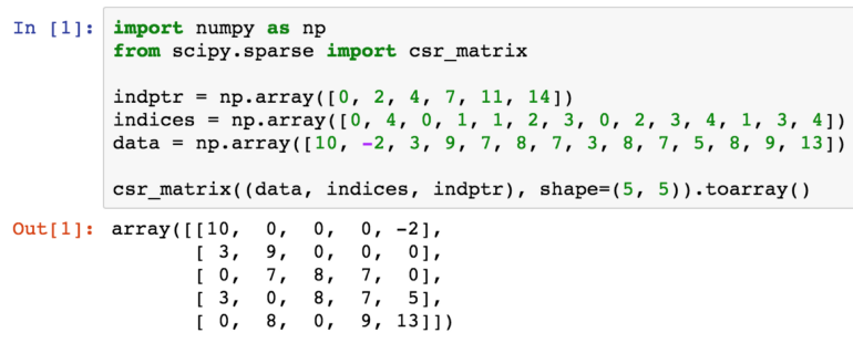
Compressed sparse row (CSR) format
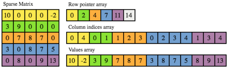
There are several formats to store a sparse matrix, such as Dictionary of Key (DOK), List of lists (LIL), Coordinate list (COO), Compressed sparse row (CSR) and Compressed sparse column (CSC). Because CSR allows fast access and matrix multiplication, it is used in SciPy Sparse matrix dot function. We borrow a nice explanation and visualization (Figure 4) of the CSR matrix from this page:
In CSR, a matrix is stored as three one-dimensional arrays of row pointers, column indices and values, where the first two are of integer type and the last one of float type, usually double. As the name suggests, non-zero entries are stored per row, where each non-zero is defined by a pair of column index and corresponding value. The column indices and values arrays therefore have a length equal to the total number of non-zero entries. Row indices are given implicitly by the row pointer array, which contains the starting index in the column index and values arrays for the non-zero entries of each row. In other words, the non-zeros for row i are at positions row_ptr[i] up to but not including row_ptr[i+1] in the column index and values arrays.
The code to initialize a SciPy CSR matrix in shown in Figure 5. Note that the shape of the matrix is needed.
sparse_dot_topn function
We implement the sparse matrix multiplication and top-n selection with the following arguments:
- n_row: number of rows of A matrix, in our case the number of names to match
- n_col: number of columns of B matrix, in our case the number of ground truth names
- Ap, Aj, Ax: pointer, index and data array of A
- Bp, Bj, Bx: pointer, index and data array of B
- ntop: top-n cosine similarity score
- lower_bound: if value of an element of C is less than lower_bound, the value will be replaced zero
- Cp, Cj, Cx: pointer, index and data array of C. C is the output matrix
void sparse_dot_topn_source(int n_row,
                        int n_col,
                        int Ap[],
                        int Aj[],
                        double Ax[], //data of A
                        int Bp[],
                        int Bj[],
                        double Bx[], //data of B
                        int ntop,
                        double lower_bound,
                        int Cp[],
                        int Cj[],
                        double Cx[])
Figure 6 Call signature of the cossim_topn function
Now we look at inside the function. First, some local variables are initiated as shown in Figure 7.
- sums: a sparse vector that records the multiplication result of the current row. It is initiated as an all zero vector.
- next: a sparse vector that keeps a linked list of the current row. Every element points to the next column index
- candidates: a list that stores all non-zero multiplication result in the current row. Top-n result will be select from candidates
- nnz: the number of non-zero elements in current row
- Cp: the row index pointer. It starts with 0.
std::vector<int> next(n_col,-1);
std::vector<double> sums(n_col, 0);

int nnz = 0;

struct candidate {int index; double value;};
bool candidate_cmp(candidate c_i, candidate c_j) { return (c_i.value > c_j.value); }
std::vector<candidate> candidates;

Cp[0] = 0;
Figure 7: Initialization of local variables in the function. “candidate” is a simple helper structure
Then, the rows of matrix A are iterated over and three main tasks are performed for every row, as indicated in Figure 8. We will analyze these one by one. In the next paragraphs, i is the current row of the loop.
for(int i = 0; i < n_row; i++){
    // Line 53-72 compute A[i, :] * B

    // Line 74-88 Use the multiplication result as the candidate list

    // Line 90-105 Select top n result of candidate list
}
Figure 8: The main loop of the function iterates over all rows of the first matrix A in the sparse matrix multiplication and performs three tasks for every row.
The first task is shown in Figure 9. It computes the multiplication of row i of matrix A with matrix B. According to the definition of CSR format, jj_start to jj_end is the range of the column index array Aj in row i. By iterating jj in line 3 in figure 9, we get all the non-zero element of matrix A on row i, i.e., j as the column of non-zero element and v as the value.
Then, we jump to the corresponding row j in matrix B (yes, still j, but now j is the row index of matrix B). kk_start to kk_end is the range of column index array Bj in matrix B, and another inner loop iterates over the non-zero elements in row j of matrix B, i.e., i is the column index, and Bx[kk] is the value.
Since we find the two elements of A[i, j] and B[j, k], the vector sums accumulates the multiplication result of A[i, j] and B[j, k] on position sums[k] (line 12 in figure 9). When the outer loop of jj and inner loop of kk finish, the sums vector stores all the multiplication result of row i.
Remember that not all the elements of the vector sums have values, many remain zero! To this end the auxiliary variables next and head are used to keep a linked list of which elements in the sums vector are non-zero. In this way, the sums vector can be quickly re-visited in next block.
int jj_start = Ap[i];
int jj_end   = Ap[i+1];
for(int jj = jj_start; jj < jj_end; jj++){
    int j = Aj[jj];
    double v = Ax[jj]; //value of A in (i,j)

    int kk_start = Bp[j];
    int kk_end   = Bp[j+1];
    for(int kk = kk_start; kk < kk_end; kk++){
        int k = Bj[kk]; //kth column of B in row j

        sums[k] += v*Bx[kk]; //multiply with value of B in (j,k) and accumulate to the result for kth column of row i

        if(next[k] == -1){
            next[k] = head; //keep a linked list, every element points to the next column index
            head  = k;
            length++;
        }
    }
}
Figure 9: Computation of A[i]*B, i.e. the product of row i of matrix A and matrix B, the first task of Figure 8.
Now, in the second task we will re-visit the sums vector and pre-select a vector candidates. The code is shown in Figure 10. Variables head and next help to jump to the next non-zero element in vector sums. We use the lower_bound input parameter here. When the result of multiplying row i of matrix A with a column of matrix B is less than the lower_bound, we ignore it, effectively setting it to zero. In the name matching case we set lower_bound to 0.5, because we do not consider cosine similarity scores lower than 0.5 anyway. Of course lower_bound can be set as the lowest possible score to disable it (In our case, the lowest cosine similarity score is zero, because all the features are positive and all feature vectors are normalized).
for(int jj = 0; jj < length; jj++){ //length = number of columns set (may include 0s)

    if(sums[head] > lower_bound){ //append the nonzero elements
        candidate c;
        c.index = head;
        c.value = sums[head];
        candidates.push_back(c);
    }

    int temp = head;
    head = next[head]; //iterate over columns

    next[temp] = -1; //clear arrays
    sums[temp] =  0; //clear arrays
}
Figure 10: Selecting the candidates for the top-n, the second task of Figure 8. Only multiplication results larger than a given lower bound are considered.
Figure 11 shows the code for the third and final task, where the top-n candidates are selected. candidates contains all the multiplication results of row A[i] with matrix B. The std::partial_sort function provides a faster way to get the top-n elements from a vector than sorting the whole vector and subsequently selecting the first n elements. If the number of candidates are less than ntop, we sort all the candidates. The top-n results are stored in matrix C.
Lines 9 to 13 transfer top-n results into matrix C. nnz is number of non-zero elements of row i in matrix C, and it can also be used as the index of Cj and Cx on the fly. In the end, we clear the candidates vector for the next loop. Finally the Cp array is updated and Cp[i+1] points to the next position.
int len = (int)candidates.size();
if (len > ntop){
    std::partial_sort(candidates.begin(), candidates.begin()+ntop, candidates.end(), candidate_cmp);
    len = ntop;
} else {
    std::sort(candidates.begin(), candidates.end(), candidate_cmp);
}

for(int a=0; a < len; a++){
    Cj[nnz] = candidates[a].index;
    Cx[nnz] = candidates[a].value;
    nnz++;
}
candidates.clear();

Cp[i+1] = nnz;
Figure 11: Selecting the top-n candidates, the third task in Figure 8. The helper function candidate_cmp is a comparator for sorting the list of candidates.
Make it callable by Python
At this point we have the C++ code all ready. Next we wrap it with Cython (Cython file is here) and call it in Python, as shown in Figure 12. The input parameters are matrix A and B, ntop and lower_bound. First, both A and B are converted to CSR format. If A and B have already been CSR format, there is no overhead in converting. Then, the number of rows of A and number of columns of B are retrieved. Next, memory for matrix C is reserved as shown in line 9 to 15. The maximum space is M*ntop elements. Before calling the C++ code, we also check some boundary condition so that zeros matrices are not input to the function.
def awesome_sparse_dot_top(A, B, ntop, lower_bound=0):
    # force A and B as a CSR matrix.
    # If they have already been CSR, there is no overhead
    A = A.tocsr()
    B = B.tocsr()
    M, _ = A.shape
    _, N = B.shape

    idx_dtype = np.int32

    nnz_max = M*ntop

    indptr = np.zeros(M+1, dtype=idx_dtype)
    indices = np.zeros(nnz_max, dtype=idx_dtype)
    data = np.zeros(nnz_max, dtype=A.dtype)

    # if A or B are all zeros matrix, return all zero matrix directly
    if len(A.indices) > 0 and len(A.data) > 0 and len(A.indptr) > 0 and \
       len(B.indices) > 0 and len(B.data) > 0 and len(B.indptr) > 0:
        cossim_topn(
            M, N, np.asarray(A.indptr, dtype=idx_dtype),
            np.asarray(A.indices, dtype=idx_dtype),
            A.data,
            np.asarray(B.indptr, dtype=idx_dtype),
            np.asarray(B.indices, dtype=idx_dtype),
            B.data,
            ntop,
            lower_bound,
            indptr, indices, data)

    # N.B. since the indices are grid id here, we still keep the shape as (M,N)
    return csr_matrix((data,indices,indptr),shape=(M,N))
Figure 12: Python wrapper.
Experiment
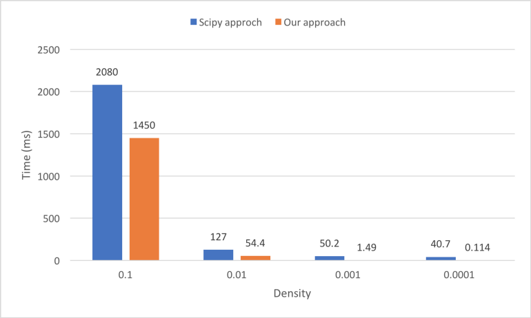
We compare two approaches to calculating the top-n similarity scores. The first is using the sparse matrices dot function followed by numpy.argpartition, as shown in Figure 13. The second is our awesome_cossim_topn function. Matrix A is 600*100000, and matrix B is 100000*800. We compare the result with different density levels 0.01, 0.001, 0.0001. We use jupyter %timeit -n 100 -r 5 to profile the run times. Table 1 and Figure 14 show the test results.
We can see the running time of SciPy approach is not linear with the density of the sparse matrix, because of the overhead of combining SciPy, NumPy and Python code. Assume the density is 0.1, our pure C++ approach is 40% faster than the SciPy approach. If the density is smaller, our approach is even faster.
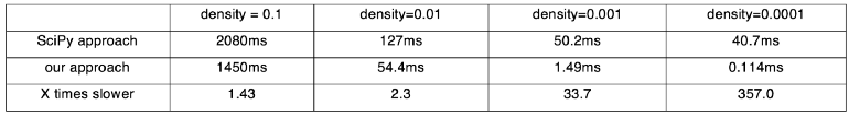
Our approach also uses less memory. In the experiment above (Matrix A is 600*100000, and matrix B is 100000*800, and suppose the type of the matrix elements is int32), some memory space is needed to store the intermediate steps of the multiplication result. The possible maximum memory usage of the SciPy approach is 600*800*4 = 1.92MB and it depends on the density of the multiplication result. In our approach, it is fixed as 12KB.
Conclusion
In this article we introduced a fast, memory efficient and elegant way to compute the multiplication of two sparse matrices and getting the top-n per row. When you have a similar task, our implementation could save you a lot of time and memory compared to using SciPy dot and np.argpartition. The code is available here. You are welcome to use it :)